Lecture 3
Stanford CS234: Reinforcement Learning | Winter 2019 | Lecture 3
recap MDP evaluation of Dynamic Programming
Dynamic Programming
- case where we know exact model (not model free)
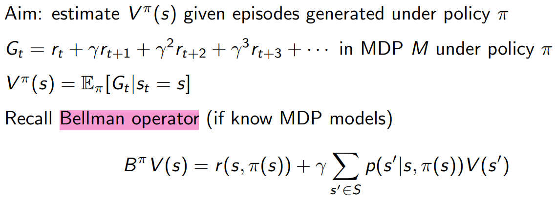
Initialize $V_0 (s)=0$ for all s
for k = 1 until convergence
for all $s$ in $S$
$V^\pi_k(s)=r(s,\pi(s)) + \gamma \sum_{s' \in S} P(s'|s,\pi(s))V^\pi_{k-1}(s')$
and we iterate until it converges → $||V^\pi_k-V^\pi_{k-1}||<\epsilon$
if k is finite
→ $V^\pi_k(s)$ is exact value of k-horizon value of state $s$ under policy $\pi$
if k is infinite
→ $V^\pi_k(s)$ is approximate value of state $s$ under policy $\pi$
→ $V^\pi_k(s)$ ← $E_\pi [r_t+\gamma V_{k-1} | s_t=s]$
resulted states of an action would be “expectation” over the state-action.

“when we know the model, we can compute immediate reward and exact estimate sum of future states. then we can substitue, instead of expanding $V_{k-1}$ as sum of rewards, we can boot strap and use current estimate $V_{k-1}$”
*Bootstrapping : 같은 종류의 예측값을 업데이트 할 때 예측값을 이용하는 것(예측값을 사용해서 예측값을 업데이트)
Model Free Policy Evaluation
we do not know the reward & dynamics model
Monte Carlo(MC) Policy Evaluation

→ we think of all the possible trajectories we can get from the policy and average all the returns
no bootstrapping
can only be applied to episodic MDPs
→ averaging over returns from complete episodes
→ requires episode to terminate
Consider a statistic $\hat{\theta}$ that provides an estimate of $\theta$ and is a function of observed data $x$ → $\hat{\theta}=f(x)$
| Definition | |
|---|---|
| Bias(편차) | ⁍ |
| Variance(분산) | ⁍ |
| MSE | ⁍ |
First-Visit MC algorithm
Initialize $N(s)=0, G(s)=0$ where $N$ is number of times a state is visited
Loop the following

$V^\pi(s)$ obtained is an ‘estimate’ thus might be wrong. So how do we evaluate??
- $V^\pi$ estimator in first-visit MC is an unbiased estimator of $E_\pi[G_t|s_t=s]$
- by law of large numbers, as $N(s)$→$\infin$, $V^\pi(s)$ converges to $E_\pi[G_t|s_t=s]$ “consistent”
Every-Visit MC algorithm
Initialize $N(s)=0, G(s)=0$ where $N$ is number of times a state is visited
Loop the following

Note there’s no “first” on this algorithm.
$V^\pi$ in every-visit MC estimator is a biased estimator
→ multiple experience on a state gets them correlated, thus data no longer ‘iid’
stiil a consistent estimator and often has better MSE
Incremental MC algorithm
we can slowly move running average in this algorithm

Non-stationary domains → dynamics model changes over time.
Advanced topic, but incredebly important in real world
MC estimate Example

Q1. Let $\gamma=1$. First visit MC estimate of V of each state?
Ans . $V_{s_1}$~ $V_{s_3}=1$ , $V_{s_4}$ ~ $V_{s_7}=0$ → we dont know states 4~7 without experience
Q2. Let $\gamma=0.9$. compare first-visit & evert-visit MC estimate of $s_2$
Ans . first-visit : 0.81 , every-visit : 0.855
→ fisrst-visit의 경우 $s_2$→$s_2$→$s_1$의 루트를 가며 첫 경험만 계산하므로
$G(s_2)=0+0.90+0.9^21=0.81$
따라서 $V^\pi (s_2)=0.81/1=0.81$이
→ every-visit의 경우 $s_2$→$s_2$→$s_1$의 루트를 가며 두 encounter 모두 계산하므로
$G(s_2)=G_1(s_2)+G_2(S_2)=(0+0.90+0.9^21)+(0+0.9*1)=1.71$
따라서 $V^\pi (s_2)=1.71/2=0.855$ 이다.
What Monte-Carlo Evaluation is doing

“approximate averaging over all possible futures by summing up one trajectory through the tree”
→ sample a return, add up all the rewards along the way
Key Limitations
Generally high variance estimator
→ Reducing variance can require a lot of data
→ Impractical when lacking data
Requires episodic settings
→ Episode must terminate to use to update $V$
Temporal Difference(TD) Policy Evaluation
Combination of Monte-Carlo & dynamic programming method
→ takes Bootstrapping aspect from dyamic programming
→ takes Sampling from Monte-Carlo
Immediately updates estimate of $V$ after each ($s,a,r,s'$) tuple → no need to wait episode to end
TD Learning estimation

→ we’re gonna get immediate reward plus discounted sum of future rewards
Now let us compare $V^\pi(s)$ of incremental every-visit MC with TD
| Incremental every-visit MC | ⁍ |
|---|---|
| TD | ⁍ |
instead of using $G_{i,t}$ we bootstrap with immediate reward plus expected future reward.
TD Error
$$
\delta_t=r_t+\gamma V^\pi(s_{t+1})-V^\pi(s_t)
$$
TD algorithm can immediately update estimated after each ($s,a,r,s'$) tuple
TD algorithm Example

Ans. [1 0 0 0 0 0 0], we can sample tuples from trajectory as below

What Temporal-Difference Evaluation is doing
$$
V^\pi(s)=V^\pi(s)+\alpha([r_t+\gamma V^\pi(s_{t+1})]-V^\pi(s))
$$

for state $s_t$, we update this by using a sample of $s_{t+1}$ to approximate expected next state distribution or future distribution. And then, we bootstrap by plugginf in previous estimate of $V^\pi$.
Evaluating Policy Evaluation Algorithms
Properties
| Dynamic Programming | Monte-Carlo | Temporal-Difference | |
|---|---|---|---|
| Usable without model of correct domain | X | O | O |
| Handles non-episodic domain | O | X | O |
| Handle non-Markovian domain | X | O | X |
| Converge to true value in limit (in Markovian domain) | O | O | O |
| Unbiased estimate of value | X | O | X |
Bias/Variance characterisics of algorithms

Batch MC and TD calculation
we might want to spend more calculation to get better estimate... for better “sample efficiency”

'ML Study > Stanford CS234: Reinforcement Learning' 카테고리의 다른 글
| Stanford CS234 Lecture 6 (0) | 2022.08.09 |
|---|---|
| Stanford CS234 Lecture 5 (0) | 2022.08.08 |
| Stanford CS234 Lecture 4 (0) | 2022.08.05 |
| Stanford CS234 Lecture2 (0) | 2022.08.05 |
| Stanford CS234 Lecture 1 (2) | 2022.08.04 |


댓글